Collection sites and site-specific characteristics

In 2015, 41 natural populations of perennial ryegrass (Lolium perenne L.) were sampled across Europe. In each population, a small number of living tillers were collected from 30–35 individual plants. The collection sites spanned areas of 100 to 290,000m², with most sites larger than 1,000m² (Supplemental Table 1). The 41 populations were collected in Belgium (BEL), Germany (DEU), Estonia (EST), France (FRA), Great Britain (GBR), Lithuania (LTU), The Netherlands (NLD), Poland (POL), Portugal (PRT) and Serbia (SRB) (Figure 1).

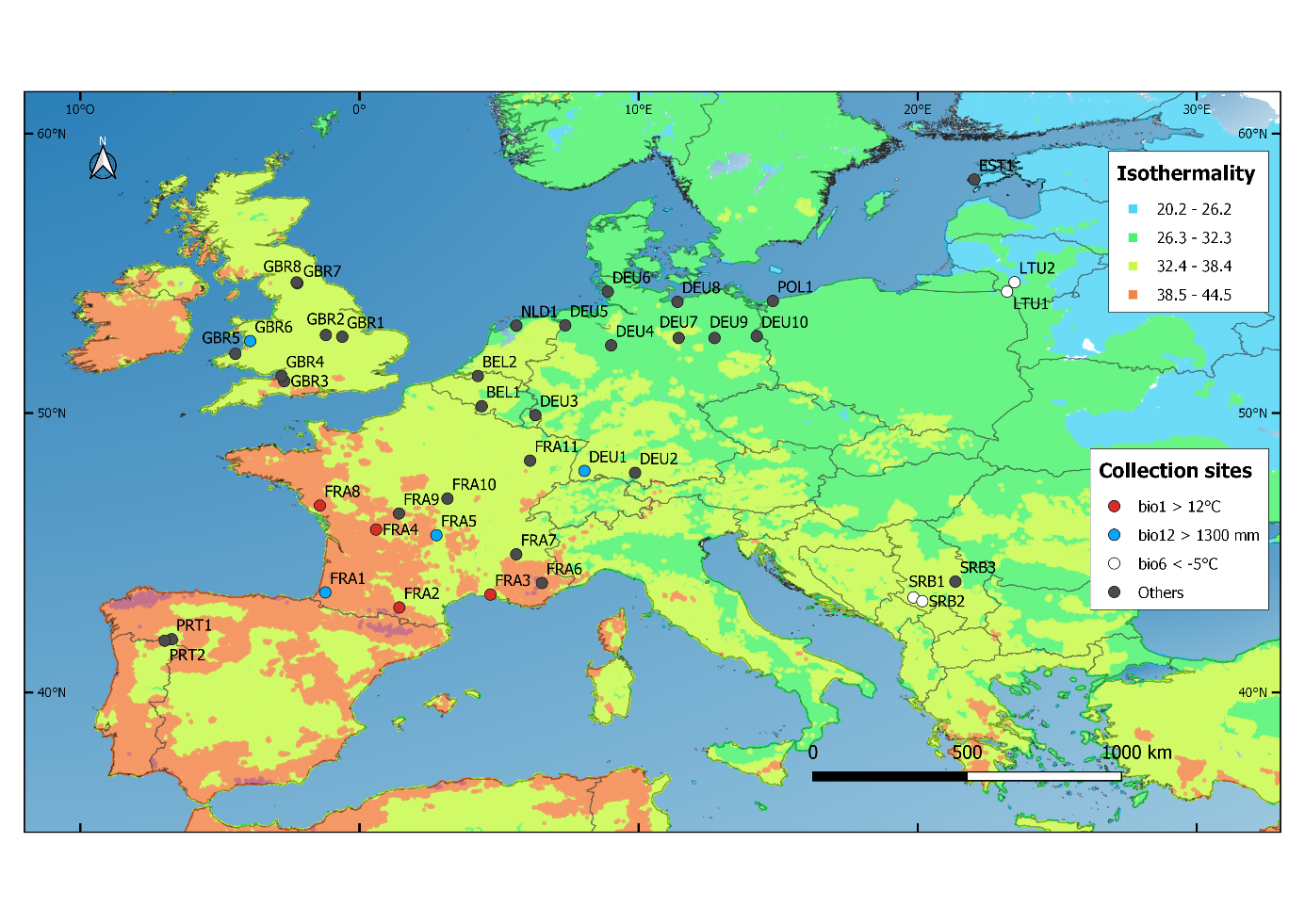
The majority of the collection sites had an elevation ranging from 0 to 800m above sea level (masl). Populations from sites above 800masl originated from Germany (DEU1, 1,040m), Serbia (SRB1, 1,076m; SRB2, 1,159m) and France (FRA5, 1,200m). The altitude of the sampling sites as well as their climatic conditions (Blanco-Pastor et al., 2021) are displayed in Table 1. The annual mean temperature (bio1) of the collection sites ranged from 5.3°C (population GBR8) to 14.8°C (population FRA3). The annual precipitation (bio12) averaged 902mm over collection sites and ranged from less than 580mm for populations DEU7, DEU9, DEU10, EST1 and FRA3, to more than 1,300mm for populations DEU1, FRA1, FRA5 and GBR6. The average daily maximum temperature of the warmest 14-day period of the year (bio5) was the highest for populations FRA3, PRT1, PRT2 and SRB3 (more than 28°C). The average daily minimum temperature of the coldest 14-day period of the year (bio6) was lowest for LTU1, LTU2, SRB1 and SRB2 (less than -5°C). Furthermore, populations EST1, FRA3 and PRT2 originated from the driest sites (precipitation <85mm in the driest quarter (bio17), Table 1).

As reported in the biological status of accessions (FAO/Bioversity, 2015) and the accession source (COLLSRC), the populations were predominantly collected from wild and semi-natural habitats (SAMPSTAT = 100, 110, 120; see Supplemental Table 1). These comprised natural grasslands, semi-natural pastures where no sowing or ploughing took place during the previous 15 to 70 years or roadsides. After collection, living tillers of the populations were transferred to the German Federal Ex Situ Genebank of the Leibniz Institute of Plant Genetics and Crop Plant Research (IPK), Satellite Collections North at Malchow/Poel, Germany for conservation. The passport data of the accessions are available via the IPK Genebank Information System GBIS (https://gbis.ipk-gatersleben.de) and are also provided in Supplemental Table 1. Individual plants within populations were pre-cultured in seedling trays using a turf-based planting substrate (Einheitserde Uetersen, Pikiererde, Uetersen, Germany) and then transferred to the field. The ploidy level on all plants grown afterwards in the experimental garden was confirmed as diploid (2x = 14) using flow cytometry at INRAE (UR P3F).

Experimental design and traits evaluated

The perennial ryegrass populations, originating from various ecogeographical conditions across Europe, were cultivated in a field trial at the Satellite Collections North station in Malchow/Poel in northern Germany (Longitude 11°28’26’’E, Latitude 53°59’40’’N, 10masl). The site is characterized by a mean annual precipitation of 544mm and a mean annual air temperature of 10.0°C over the past 10 years. The predominant soil type is a sandy loam. The trial was set on a 38m × 18m field plot with homogeneous soil conditions. Plants were transplanted to the field and arranged in a completely randomized design on 24 September 2015 (except for plants from populations collected in Great Britain, which were transplanted on 23 October 2015 and for populations DEU8 and DEU10, which were too weakly developed and were transplanted in March 2016). One clone of each originally sampled individual plant was randomly distributed in the field trial area without replication, except three plants per population, which were set up in two replicates (clones). A number of clonal replicates were planted in April 2016, as indicated in Figure 2, because they were too weakly developed in September 2015. Spacing between the individual plants was 45 × 50cm. An equalisation cut was made at the beginning of the growing season in 2016 after recording the winter damage score. Three (2016) and four (2017) harvest cuts were completed, and fertilizers were applied after each cut, amounting to 240kg N/ha per year as calcium-ammonium-nitrate (Table 2). A weather station located at the Satellite Collections North recorded the local weather conditions at the experimental site (Supplemental Table 3). The first winter after planting was characterized by mild temperatures in November and December (7.7 and 7.1°C average daily temperatures, respectively). January was cold, with an average monthly temperature of -0.6°C (long-term average (1991–2020): 1.5°C in January in Kirchdorf/Poel (DWD, 2023)) and 11 days with minimal temperatures below -5.0°C, followed by a very dry spring with only 9.1mm rainfall in April 2016 (long-term average (1991–2020): 32.0mm in April in Kirchdorf/Poel (DWD, 2023)). The experimental year 2017 was characterized by average air temperatures but high rainfall in June and July (Supplemental Table 2).

The following traits were visually scored on a scale of 1 to 9 by an experienced genebank worker during the three experimental years of the trial: winter damage (WID), growing in spring (GSp), summer growth (GSu), growing before winter (GWi) and general disease susceptibility (DIS) (Table 2). Growth parameters were assessed from a visual impression of the aboveground biomass of the plant three times in each year: in April (GSp), in August (GSu) and before winter in October (Gwi) expressed on a scale from 1 (low biomass) to 9 (strong biomass). WID describes the extent of the visually detectable damage after winter (proportion of dead tissues) on a scale from 1 (low damage) to 9 (strong damage). DIS rates the severity of the disease occurrence on the basis of visually detectable leaf damage from 1 (low susceptibility) to 9 (high susceptibility). This score gives an overall visual impression of disease infection and does not differentiate between pathogens. Heading date (HAE) of plants was recorded in 2016 and 2017 as the number of days from the first of April to the day when the tips of five ears were visible. Natural plant height was measured in spring (SPH) before the first cut using a herbometer (HerboMETRE Electronique, Framstore, France). Plant height was measured again about 10 days after the first cut and is referred to as regrowth (REG_1), i.e. the capability to recover quickly and to develop new biomass after cutting. Plant height was measured again before and after the second cut in July. The plant height 10 days after the second cut (REG_2) now gives information about the regrowth capability after the summer cut. Height increment (HgtIn) was calculated by subtracting REG1 from the height measured before the second cut (HSC) and serves as a measure of the strength of biomass growth between the cuts. Finally, tussock size was measured several times throughout 2016 and 2017 using a ruler. Tussock size was calculated as the mean of two perpendicular measurements of plant width; the highest value over recorded dates in 2016 and 2017 was used for data analysis (Table 2).

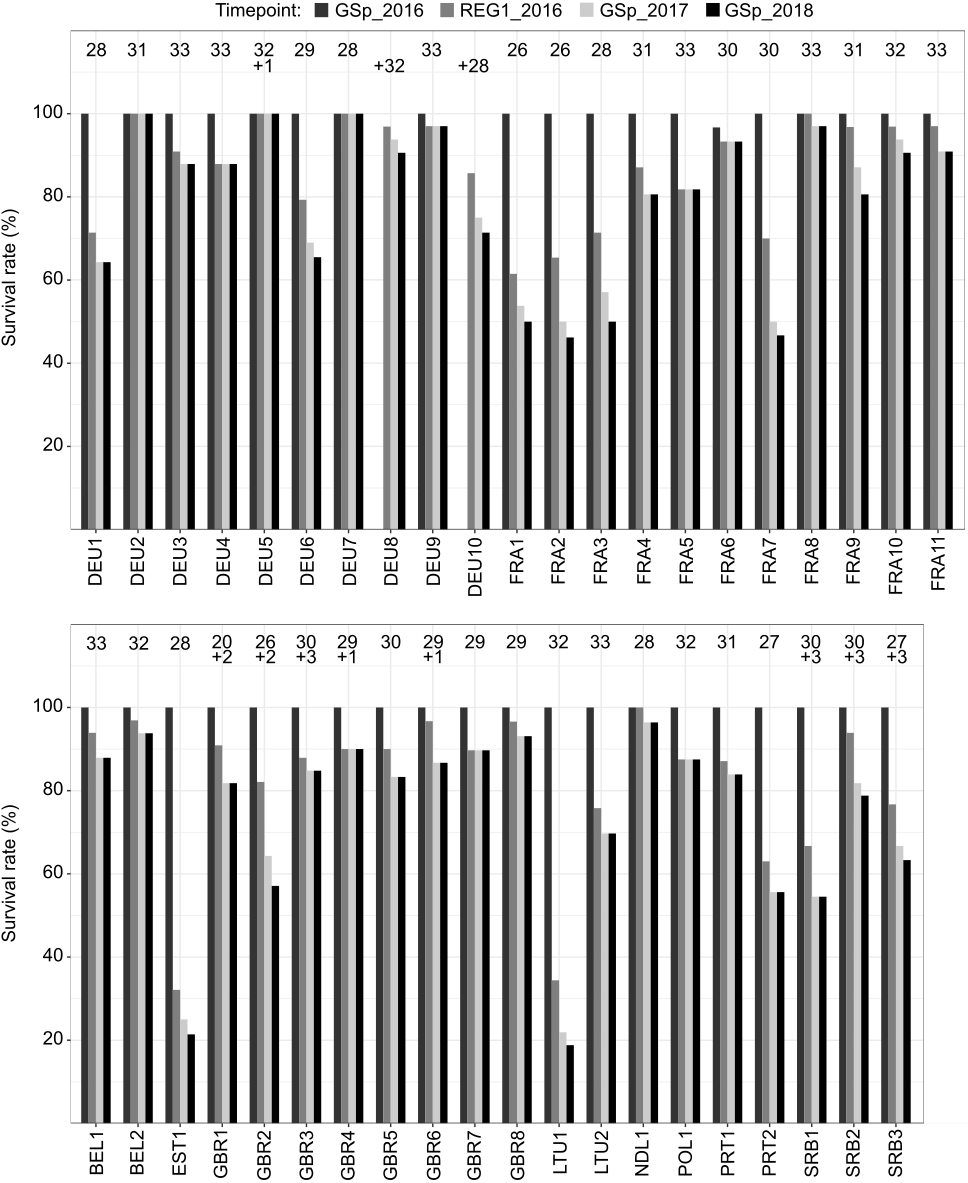
The number of living plants per population was counted 50 days after first planting date and at four later time points: (1) in spring 2016 (date of record of GSp in 2016) in order to determine survival after the first winter, (2) after heading and first cut (date of record of REG1 in 2016), (3) in spring 2017 (date of record of GSp in 2017) to determine survival after the second winter and (4) in spring 2018 (date of record of GSp in 2018) as an indicator of persistency. The number of living plants at the different record dates was expressed as a percentage of the number of plants counted 50 days after the first planting date to exclude weak plants that died right after the planting, plus later planted individuals.

Statistical analysis

The Software R (R Core Team, 2020) was used for statistical analyses. Data processing only included plants surviving the second experimental year and populations with more than 15 surviving plants. This number is based on our considerations of finding a compromise between the minimum number of plants that must have survived to calculate a reliable population mean, and ensuring that the variance model does not become too unbalanced. At the same time, we wanted to avoid excluding too many populations from further analysis, as this would result in the loss of information. Therefore, we set a threshold of at least 15 surviving plants per population, corresponding to at least 50% of the total plants/genotypes.

To test for outperforming populations, a one-way analysis of variance (ANOVA) with population as fixed effect was applied for each trait in each year. Data across all populations were visually checked for normal distribution using Q-Q-plot and the Lillie test (Gross & Ligges, 2015) and for variance homogeneity using the Levene test of the package ‘car’ (Fox & Weisberg, 2011). Population means were estimated with the ‘lsmean’ function and compared to the grand mean using the command ‘eff’ (Lenth, 2016). Populations were considered significantly different from the grand mean if p ≤ 0.05. If variance homogeneity was violated, the vcovHC function (Heteroscedasticity-Consistent Covariance Matrix Estimation) of the package ‘sandwich’ (Zeileis, 2004) was applied for post hoc comparison.

For multivariate analysis, for each trait, population means were standardized (i.e. centred and reduced). Euclidian distances between populations and between traits were calculated using the standardized population means and the ‘dist’ function of base R. Clustering of the populations based on the recorded phenotypic traits was visualized in a heatmap generated with the ‘heatmap.2’ command of the ‘gplots’ package (Warnes et al., 2020).

Values of populations for agronomic traits were correlated to values of bioclimatic variables and geocoordinates at their sites of origin and with each other (Pearson’s correlation coefficient of the R package ‘Hmisc’ (Harrell, 2021)). Correlations were considered significant if p ≤ 0.05. Climate norms (period 1989–2010) of bioclimatic variables similar to the BIOCLIM variables usually derived from the WorldClim – Global Climate Database, were used. They were already presented in Blanco-Pastor et al. (2021) and are also described in Supplemental Table 2. Fifteen BIOCLIM-like variables were included in the correlation analysis.

Survival rate

In all populations, the plants survived the first winter without major losses as indicated by the high survival rates in spring 2016 (date of record of GSp_2016), which ranged from 96 to 100% (Figure 2). Of the additional, later planted individuals of DEU5, GRB1-4, GRB6 and SRB1-3, all but one each of SRB1, SRB2 and SRB3 survived until the end of the trial. No survival rate is available for the first winter for populations DEU8 and DEU10, because the respective genotypes could not be planted before March 2016. The highest losses of plants were recorded after the first cut of 2016. The survival rate at the date of record (REG1_2016) clearly declined for some populations to less than 70%, but these populations then stabilized, with no further dramatic losses in the following years. The populations EST1 and LTU1 showed the highest losses at this timepoint, followed by FRA1, FRA2, PRT2, FRA3, DEU1, FRA7 and SRB1. A high survival rate at the end of the 3-year experiment was recorded for populations FRA8, DEU2, DEU5, DEU7, DEU9 and NLD1, of which > 95 % of the cultivated plants survived (Figure 2).

Phenotypic characterization of the populations

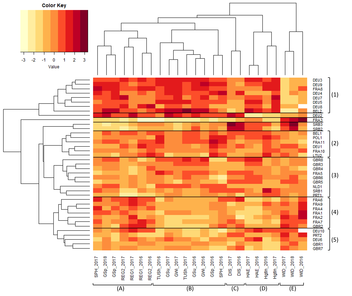
The phenotypic diversity between populations was analyzed by a doubled cluster analysis on recorded traits and on populations. Eleven phenotypic traits were measured in two or three consecutive years, resulting in 24 combinations of traits and year of record (Table 2, Supplemental Tables 4 and 5). The cluster analysis on standardized population means grouped these 24 trait × year combinations into five major groups (Figure 3). The most outstanding phenotypic cluster E contained the ordinal trait winter damage recorded in all three years. Heading date and height increment between the first and second cut for both years grouped together in cluster D, while the two disease susceptibility ratings formed a separate cluster C. Plant height in spring and growth in spring in 2016 were in cluster B together with growth in summer and winter and tussock size (GSu, GWi, TUSh). The plant height in spring in 2017 and growth in spring in 2017 and 2018 formed cluster A together with the two measured regrowth heights in 2016 and 2017.

Two populations with low survival rates (EST1 and LTU1) were not included in the cluster analysis. The 39 remaining populations were assigned to five main clusters (Figure 3). Cluster 1 contained eight outstanding populations predominantly originating from Germany but also from France and Belgium. These were characterized by exceptionally low winter damage and strong and vigorous growth as indicated by high values (dark red colour) for these variables (SPH, GSp, REG, TUSh, GSu, and GWi, Figure 3). Population DEU2 was close to this cluster but had a later heading date (HAE) and a lower height increment (HgtIn). All the other populations were grouped along another branch of the clustering tree. An outstanding population was FRA3 with high winter damage and low values for the other variables. Cluster 2 (six populations from the north-eastern and central regions of the sampling area across Europe) and Cluster 3 (nine populations including five populations from Great Britain) differed for growing in spring and plant height in spring in 2016, but revealed no clear pattern for the other traits. SRB2 and SRB3 were separated from them by less vigorous growth but higher disease susceptibility and higher winter damage. Cluster 4 contained one British and six French populations and showed high winter damage (Cluster E) which was compensated for by a high spring and summer growth (GSp, GSu, Cluster A). All five populations belonging to Cluster 5 showed relatively high winter damage and low performance in all the other traits (Figure 3).

Winter damage, growth in spring, growth before winter and heading date presented almost similar value ranges in the three trial years, while growth in summer and disease susceptibility fairly differed between the years (Table 3). With a year-dependent average score of 5.4 to 6.1, winter damage was on an intermediate level, with the strongest damage after winter 2017. Data from the three consecutive years indicated that populations from France generally had the highest winter damage in 2016 and 2017, in particular populations originating from southern France (FRA1-FRA4) (Figure 3, Table 3, Supplemental Table 4 ). Populations from Great Britain (GBR3, GBR7), Serbia (SRB2, SRB3) and Portugal (PRT2) also showed high winter damage. Populations with the lowest winter damage originated from Germany, but also from Belgium (BEL2), France (FRA11) and Lithuania (LTU2). The mean value of growth in spring ranged from 4.2 to 4.8 according to years. Populations with strong growth in spring were BEL2, FRA8 and several German populations, in particular DEU9. In contrast, the material from Serbia exhibited low spring growth, particularly in 2017 and 2018. Related to their late planting in 2015, also the British populations showed low spring growth. Population FRA3 differed from all the other populations by revealing the highest winter damage and the lowest growth in spring in all three experimental years.

Growth in summer, i.e. the biomass development of the plants in August after the two cuttings, was stronger in 2016 than in 2017. Outstanding populations with very strong growth in summer were BEL2, FRA8, DEU2, DEU3 and DEU9. Growth before winter reached rather similar values in both years. Well-developed plants with a high growth performance before winter were observed in populations BEL2, FRA8, DEU2, DEU3, DEU7 and DEU9. The average heading date was 47.0 and 48.5 days in the two years. Late types (HAE > 57 days) originated from Belgium, in particular, BEL2 with 67 days in 2017, northern Germany (DEU5-10) and northern Britain (GBR8). Although collected close to the site of GBR8, heading date of GBR7 was much earlier. Next to several French populations, DEU2 revealed the earliest heading date in the whole set with only ~25 days after 1 April in both years. General disease susceptibility, scored in September or October, reflected the general leaf health under the infection with several diseases. On average, the disease infestation was higher across populations in 2016 than in 2017. In particular FRA6, DEU2 and two out of three populations from Serbia (SRB2 and SRB3) showed a higher disease susceptibility than the other populations, even in 2017 when disease pressure was lower. Generally, based on all scored traits, BEL2, FRA8, DEU3 and DEU9 exceeded the performance of all other populations. Additionally, DEU2 revealed good biomass scorings throughout the experimental time, but tended to a higher disease susceptibility. DEU2 and DEU3 were both among the best populations for all scored traits, but strongly differentiated in heading date, with DEU2 as an early heading type and DEU3 as a late type with an average of 60 days to heading. The weakest population was FRA3, characterized by the strongest winter damage, the lowest spring and summer growths as well as the least developed plants before winter (Supplemental Table 4).

Plant height and diameter were measured at several time points during the experiment. On average across populations, plant height in spring, regrowth height after first cut and tussock size were higher in 2017 than in 2016, while regrowth height after second cut had similar average values in the two years. In contrast, height increment, as a measure of plant height development between first and second cuts, was only about half as high in 2017 as in 2016 (Table 3). The spring height measurements confirmed the findings from growth in spring scorings. The average plant height in spring was 125mm in 2016 and increased to 205mm in 2017. Populations with large spring heights were mostly from France (FRA4, FRA6, FRA8, FRA11) and Germany (DEU2, DEU4, DEU8, DEU9). Similar to growth in spring scorings, spring height was exceptionally low for all the material from Great Britain, particularly in 2016, and for material from Serbia (Figure 3, Supplemental Table 5). Regrowth height 10 days after the first cut reached 137mm on average across populations in 2016 and 196mm in 2017. Populations with strong regrowth after the first cut were FRA7, FRA8, FRA9 and DEU1, DEU2, DEU3, DEU8 and LTU2. Populations from PRT and SRB generally revealed a slow regrowth after the first cut. The regrowth height 10 days after the second cut was as on average 183mm and rather stable between the two years. The population with regrowth height after second cut stronger than most of the other populations, considering both years, originated from Germany (DEU3, DEU5, DEU7, DEU8, DEU9) and France (FRA8). In contrast, regrowth capability below that of most of the other populations was measured for populations from Portugal (PRT1), Serbia (SRB2) and France (FRA3). The increment of plant height, expressed as the height difference from regrowth height after first cut to the height at the second cut, declined on average across populations from 147mm in 2016 to 92mm in 2017. Outstanding populations with a high height increment in both years and a late spring growth were DEU9 and FRA8. Tussock size of the individual plants averaged 206mm at the end of 2016 and increased on average by 50mm by the end of 2017. Highest tussock sizes (> 290mm) were generally recorded for the strong growing populations such as BEL2, FRA8, DEU3, DEU4, DEU5 and DEU8, while most populations from France, Portugal and Serbia had tussock sizes below 230mm.

Relation between performances of populations and bioclimatic variables at their sites of origin

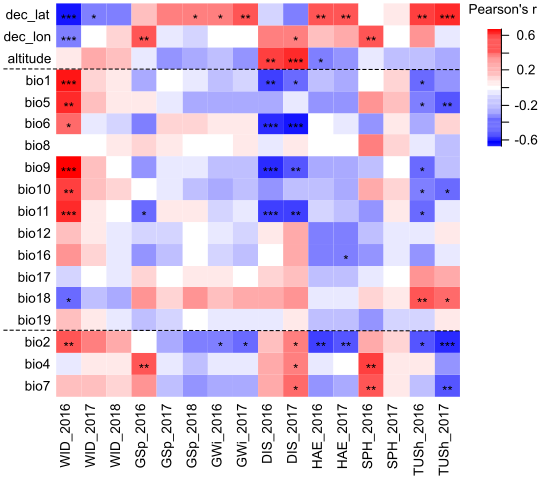
Correlations between the phenotypic traits of the populations and the climatic variables at their sites of origin are displayed in Figure 4. Among all phenotypic traits, winter damage in 2016 highly correlated with almost all climatic variables. Winter damage in 2016 showed the highest correlations with the mean annual temperature (bio1, r = 0.59, p < 0.001) and mean temperature in the driest quarter (bio9, r = 0.67, p < 0.001). The temperature daily range correlated with the susceptibility of the populations to cold winters as indicated by the correlation between winter damage in 2016 and temperature diurnal range (bio2, r = 0.45, p < 0.001). However, correlations were weaker and not significant in the following years. Growth in spring correlated negatively with minimum temperatures during cold seasons (bio11, r = -0.40, p < 0.05), but only for 2016. Hence, the lower the temperature during the winter period at the site of origin, the stronger was the plant growth in spring after transplanting. Furthermore, temperature seasonality (bio4) was positively correlated with growth in spring 2016 with r = 0.42 (p < 0.01). Days to heading correlated little with bioclimatic variables, except for mean diurnal range in both experimental years (bio2, r = -0.46, p < 0.01/-0.43, p < 0.01, Figure 4).

Tussock size in both years correlated negatively with bio2 (r = -0.40, p < 0.05/-0.55, p < 0.001). Disease susceptibility in both years correlated negatively with several temperature variables but not with precipitation indices. The lower the average daily minimum temperature (bio6, r = -0.53, p < 0.001/-0.57, p < 0.001) and the lower the mean temperature of the coldest quarter (bio11, r=-0.51, p<0.001/-0.48, p < 0.01), the higher was the damage caused by diseases in the field experiment. Accordingly, the higher the altitude of the site of origin, the higher the disease susceptibility in both years (r = 0.48, p < 0.01/0.53, p < 0.001). The latitude of the site of origin correlated positively with heading date, growth before winter and tussock size and negatively with winter damage in 2016 and 2017. Other phenotypic traits showed only low correlations with the basic climate norms (Figure 4).